We’ve just added Gnina-based scoring (pronounced NEE-na) [Publication] to Boltzmann Maps — giving you another way to evaluate docking poses, side-by-side with tools like Vina, DiffDock, BMaps, and OpenMM.
Gnina extends the Vina/Smina framework with deep-learning models trained on experimental protein–ligand complexes. Instead of relying only on force-field heuristics, it predicts binding affinity from the 3D structure of a complex — using a CNN trained to recognize patterns seen in real-world binders.
Why Add Gnina?
It helps you rank, cross-check, and triage poses with an extra layer of insight.
- Rescoring: Use Gnina to prioritize realistic poses from any method — Vina, DiffDock, or your own.
- Pose selection: If both Gnina and your docking method favor the same pose, you have a stronger case to move it forward.
- Hit enrichment: Combine Gnina with OpenMM minimization to pull the most plausible binders to the top of your list.
Gnina doesn’t replace traditional scores — it complements them. And in Boltzmann Maps, you can see them all in one place.
Use Cases Inside BMaps
With Gnina energies now built into Boltzmann Maps, you can:
- View Gnina scores alongside docking scores, minimization energy, fragment maps, and water networks.
- Run scoring on any pose set — from DiffDock, Vina, or elsewhere.
- Filter, rank, and prioritize analogs or fragments with multiple scoring channels.
Example: Using Gnina Metrics to Gain Confidence and Find New Fragment Growing Opportunities
Here we are looking at different poses of the ligand 3TE bound to the sirtuin-2 protein 4RMG. Six poses were found using DiffDock and minimized within the protein environment using the OpenMM minimizer supported in BMaps and scored according to the BMaps interaction score calculator. These are labeled 3TE_[1-6], whereas the crystal bound ligand is 3TE.1:X
As our goal is to determine if there are any poses we may prefer to analyze over or alongside the crystal ligand pose, we turn to the Compound Table where we can compare calculated values for each compound. Rapid Gnina energy calculations are run automatically in the background and are ready by the time we open the Compound Table.
In the Compound Table we compare the Interaction Score vs three Gnina calculated values:
- Gnina Pose Score – Gnina’s predicted probability that the pose is within 2Å of the correct binding pose [Best Value: 1.0]
- Gnina Affinity – Gnina’s prediction of binding affinity in pK units (6 = 1 µM, 9 = 1 nM) [Higher is better]
- Gnina Stress – Intramolecular energy calculated by Gnina [More negative is better]
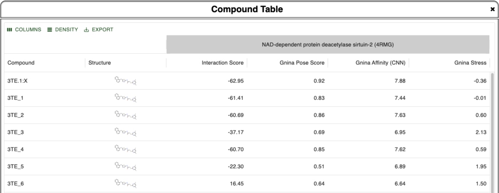
Figure 1. Compound Table in Boltzmann Maps showing metrics for comparison against the crystal ligand and 6 different DiffDock derived and BMaps minimized poses.
From this we are instantly convinced that our crystal pose is the best pose we have been able to find as all four metrics align to show this. In addition, we see that 3TE_1 is pretty close in metrics across the board as well, so if its pose is unique, it may provide additional binding site or binding mode opportunities. Note that because we used DiffDock to perform docking and as DiffDock is a global protein docker, the docked poses may be in different sites, not just the same site as the crystal pose.
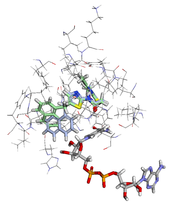
Figure 2. Ligand View of 4RMG PDB in BMaps with NAD (grey), crystal ligand 3TE.1:X in green and docked and minimized pose 3TE_1 in light blue. 3TE_1 naphthalene is rotated towards NAD and is exposed to additional pocket space as compared to the crystal ligand naphthalene.
Looking at the two ligand poses, 3TE.1:X our crystal pose in green, and 3TE_1 our docked pose in light blue, we see that the difference between their poses is almost entirely the rotation of the dihedral between the 1,3-thiazole and the naphthalene. While the crystal pose has more of a chance to interact with the aromatic ring of the phenylalanine in SIRT-2 through a t-pose pi-pi interaction with the naphthalene, our pi-pi tool indicates that interaction is not currently occurring. Meanwhile, the 3TE_1 naphthalene pose comes much closer to forming a good hydrogen bonding angle with the hydroxyls of the interacting NAD and also gives us better access to open areas in the pocket for potential fragment growing. Indeed a fragment grow in the now accessible pocket reveals 26 fragments with binding scores that may improve the overall ligand affinity.
Comparing this newly grown fragment in the Compound Table against our crystal ligand, we see we have improved across Interaction Score and Gnina Affinity, while Gnina Pose Score and Gnina Stress indicates to us that this structure is significantly more stressed than the crystal ligand which may affect its binding stability in the pocket. We also notice that this structure is stabilized by two new pi-pi interactions with the protein which may help to overcome the penalty from the stress and also indicate a partial reason for the improved Interaction Score and Gnina Affinity.

Figure 3. Easy comparison across Gnina and Bmaps metrics in the BMaps Compound Table for crystal ligand 3TE.1:X and fragment grown compound from 3TE_1, here called 3TE_7. Table shows improved Interaction Score and Gnina Affinity and less good Gnina Pose Score and Gnina Stress.
By having the additional Gnina scoring metrics we were therefore able to gain confidence in the results of triaging alternative poses from our crystal ligand, leading to the discovery of a fragment growing opportunity to improve ligand binding. We also find the Gnina scores helpful in evaluating the results of our fragment growing opportunities to guide us towards further improvements throughout the design process as well as warn us of potential energetic liabilities that fragment grown structures may have.
Built for Comparison
Gnina fits naturally into BMaps, and as we saw with our example, using multiple methods and comparing them directly in the Compound Table can build more trust in your results than any single score could.
Here is a typical workflow:
- Dock (Vina, DiffDock, etc.)
- Minimize the ligand
- Score with Gnina – Done automatically
- Quickly overview results in the Energies tab
- Filter and sort using the Compound Table for deeper analysis
This makes it easier to spot strong candidates — and weaker ones — before investing in synthesis or simulations.
Move faster and design smarter with Gnina scoring available now in Boltzmann Maps.
Sneak Preview: Gnina Docking will be available in a couple of weeks!
Thank you to the authors of Gnina. You can find their publication and Github repo here:
McNutt, A.T., Francoeur, P., Aggarwal, R. et al. GNINA 1.0: molecular docking with deep learning. J Cheminform 13, 43 (2021). https://doi.org/10.1186/s13321-021-00522-2